Mean Field Theory and Solar Dynamo Modeling

In a recent post, I talked about the characteristics of the sun’s 11 and 22 year cycles, the observed laws which describe the behavior of the sunspot cycle, how proxy data is used to reconstruct a record of solar cycles of the past, Grand Solar Maxima and Minima, the relationship between Total Solar Irradiance (TSI) and the sunspot cycle, and the relevance of these factors to earth’s climate system. In a follow up post, I went over the structure of the sun, and some of the characteristics of each layer, which laid the groundwork for my last post, in which I explained the solar dynamo: the physical mechanism underlying solar cycles.

Before elaborating on the sun’s role in climate change in the installment following this one, I’ll be going over an approach called “Mean Field Theory” in this installment, which dynamo theorists and other scientists sometimes use to make the modelling of certain systems more manageable. As was the case with part III, this may be a bit more technical than most of my subscribers are accustomed to, but I think the small subset of readers with the tools to digest it will appreciate it. And to be perfectly blunt, writing this was not just about my subscribers. I wanted to do it. It was an excuse for me to dig more deeply into something that has been going on in modern stellar astrophysics that I thought was interesting. The fact that it happened to be tangentially related to my series on climate science was a mere convenience. Anyone wanting to avoid the math and/or to cut to the chase with respect to the effects of solar cycles on climate change might want to skip ahead to part V, or perhaps just read only the text portions of this post. However, for those who don’t mind a little bit of math, I present to you the following:

Mean Field Theory

One approach by which scientists and mathematicians can simplify the models describing large complex systems stochastic effects is called Mean Field Theory (Schrinner 2005). This involves subsuming multiple complicated interactions between different parts of a system into a single averaged effect. In this way, multi-body problems, (which are notoriously difficult to solve even with numerical approximation methods with supercomputers), can be reduced to simpler single body problems. For instance, the velocity field u and magnetic field B could each be broken up into two separate terms: A mean term (u₀ and B₀ respectively), and a fluctuating term (u’ and B’ respectively), whereby the mean terms are taken as averages over time and/or space depending on what is appropriate to the system being modeled.

In other words, u = u₀ + u’ and B = B₀ + B’, where (by definition) the average velocity <u> = u₀, the average magnetic field <B> = B₀, because u₀ and B₀ are the mean field terms, and the average of the fluctuating terms <B’> and <u’> are both equal to zero by definition. The angled brackets simply denote a suitable average of the term they enclose (again taken over time and/or space as deemed appropriate by the scientist or mathematician). The reason the fluctuating terms average out to zero is because the mean field terms are defined as the average of the entire field, so by definition, the only way that can be true is if the fluctuating terms average out to zero.

Using the vector calculus identity ∇ × (∇ × B) = ∇(∇·B) + ∇²B, and the fact that ∇·B = 0 by Gauss’s Law for magnetic fields, the induction equation, ∂B/∂t  = ∇ × (u × B − η∇ × B) from the previous section can also be expressed as ∂B/∂t = η∇²B + ∇ × (u × B), where ∇²B is called the Laplacian operator of the magnetic field B.

Plugging in our mean field equations u and B into this form of the induction equation:

∂B₀/∂t + ∂B’/∂t = η∇²B₀ + η∇²B’+

∇ × (u₀× B₀) + ∇ × (u₀ × B’) +

∇ × (u’ × B₀) + ∇ × (u’ × B’)

Now we take the average of both sides:

∂<B₀>/∂t + ∂<B’>/∂t = η∇²<B₀> + η∇² <B’> + 

∇ × <u₀× B₀> + ∇ × <u₀ × B’> +

∇ × <u’ × B₀> + ∇ × <u’ × B’>

However, we’ve already know that <B₀> = B₀, <u₀> = u₀, and <u’> = < B’> = 0, so this can be simplified:

∂B₀/∂t = η∇²B₀ + ∇ × <u₀× B₀> + ∇ × <u’ × B’>.

The ∇ × <u’ × B’> is typically then replaced with a term ∇ × ε, where ε is called the mean electromotive force (Radler 2007). This yields the Mean Field Induction Equation:

∂B₀/∂t = η∇²B₀ + ∇ × <u₀× B₀ + ε>

Although many details of the theory are still being worked out, models based on the solar dynamo mechanism are consistent with the periodicity of the solar cycle, Hale’s law (the opposing magnetic polarity of sunspots above and below the solar equator and the alternation of polarity in successive 11 year cycles), as well as both Sporer’s and Joy’s laws (the apparent migration of sunspots towards the equator as a cycle progresses, as well as their tilt), which together produce the observed sunspot butterfly diagrams I talked about here.

Some models can even simulate variations in amplitude from one cycle to the next, but the precise manner in which Grand Solar Maxima and Minima emerge is still being worked out. Consequently, our models’ ability to reliably and accurately forecast them is currently still limited. Methods have been developed for estimating sunspot number and solar activity of a cycle’s solar maxima from observations of the poloidal field strength of the preceding cycle’s solar minima (Schatten 1978, Svalgaard 2005). In addition to only providing information on the solar maxima immediately after the minima being measured, this approach is also limited by the fact that our poloidal field measurements only go back a few cycles, and because the poloidal magnetic fields during solar minima are difficult to measure reliably, because they are weak and have radial as well as meridional components.

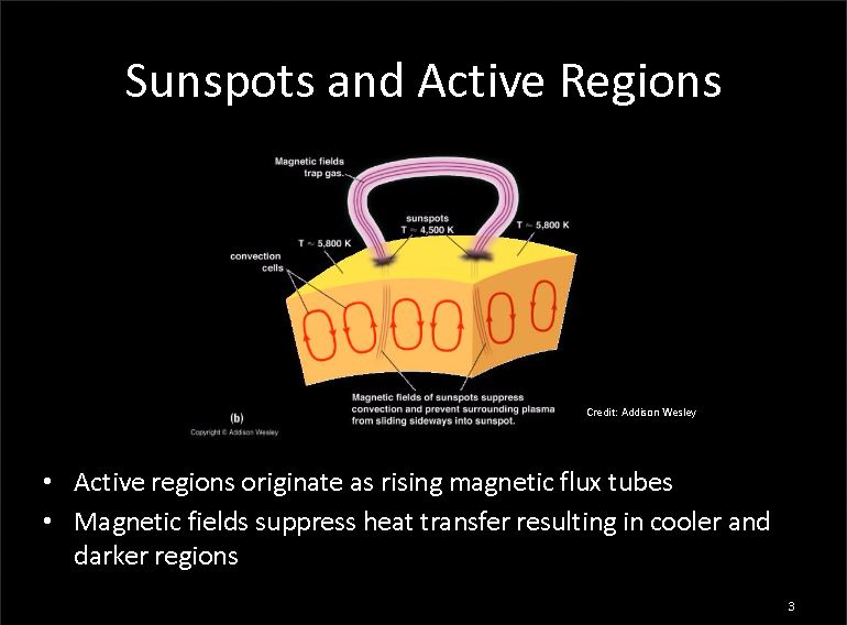
Other researchers have focused on kinematic flux transport solar dynamo models which, in addition to differential rotation, include the effects of meridional flow in the convective envelope, whereby the poloidal magnetic field is regenerated by the decay of the bipolar magnetically active regions subsequent to their emergence at the solar surface (Dikpati 1999, Dikpati 2006, Choudhuri 2007). Active regions are the high magnetic flux regions at which sunspots emerge.

Image  by Andres Munoz-Jaramillo (check out his fantastic presentations on solardynamo.org).

This meridional flow sets the period of the cycle, the strength of the poloidal field, and the amplitude of the solar maximum of the subsequent cycle. However, estimates of meridional flow velocities prior to 1996 are highly uncertain (Hathaway 1996). All of these models have been criticized by peers of their proponents. A concise summary of the blow by blow can be viewed here.

As for Grand Solar Maxima and Minima, no comprehensive theory has yet emerged on how they arise and decay, let alone a scientific consensus. However, certain constraints have been identified. There is evidence that the dynamo cycle does continue in some modified form during Maunder-type minima periods. The idea is that the dynamo enters Grand Maxima and Minima by way of chaotic and/or stochastic processes. In the case of Grand Maxima, the dynamo also exits that state via stochastic processes. In the case of Grand Minima, on the other hand, the dynamo then gets “trapped” in this state, but eventually gets out of it via deterministic internal processes (Usoskin 2007). It is also thought that the polarity of the sun’s toroidal magnetic field may lose its equatorial anti-symmetry during such minima, and instead become symmetric (Beer, Tobias and Weiss 1998).

Truly fantastic long term predictive power for solar cycles probably won’t be achieved until poloidal magnetic field generation is better understood, which will likely include improvements in flux transport models, and a more complete characterization of the statistical properties of bipolar magnetic regions (BMRs). For a comprehensive overview of the current state of Solar Dynamo Models and their predictive strengths and limitations, see Charbonneau 2010.

In the next installment, I’ll explain how all of this relates to climate change on earth, and address the elephant in the room: “are solar variations responsible for the current global warming trend?”

Related Articles:

• How Continental Drift affects Climate: Part I – Plate Tectonics, Albedo, and the SnowBall Earth Hypothesis
• How Continental Drift affects Climate: Part II – Possible Snowball Earth Triggering Mechanisms + Regional Effects of Mountain Ranges
• Milankovitch Cycles and Climate: Part I – Axial Tilt and Precession
• Milankovitch Cycles and Climate: Part II – Orbital Eccentricity, Apsidal Precession and Orbital Inclination
• Milankovitch Cycles and Climate: Part III – Putting it All Together
• The Climatological effects of Volcanic Eruptions: The End Permian Extinction, the Toba Super-Volcano, and the Volcanic Explosivity Index
• The Ultimate Environmental Cataclysm: Asteroid and Comet Impacts and their Effects on Climate
• The Sun and Earth’s Climate: The Solar Cycle and the Maunder Minimum
• The Structure and Properties of the Sun
• The Solar Dynamo: The Physical Basis of the Solar Cycle and the Sun’s Magnetic Field

References:

Beer, J., Tobias, S., & Weiss, N. (1998). An active Sun throughout the Maunder minimum. Solar Physics, 181(1), 237-249.

Charbonneau, P. (2010). Dynamo models of the solar cycle. Living Reviews in Solar Physics, 7(1), 1-91.

Choudhuri, A. R., Chatterjee, P., & Jiang, J. (2007). Predicting solar cycle 24 with a solar dynamo model. Physical review letters, 98(13), 131103-131103.

Coriolis, G. G. (1835). Théorie mathématique des effets du jeu de billard. Carilian-Goeury.

Dikpati, M., & Charbonneau, P. (1999). A Babcock-Leighton flux transport dynamo with solar-like differential rotation. The Astrophysical Journal, 518(1), 508.

Dikpati, M., De Toma, G., & Gilman, P. A. (2006). Predicting the strength of solar cycle 24 using a flux‐transport dynamo‐based tool. Geophysical research letters, 33(5).

Hathaway, D. H. (1996). Doppler measurements of the sun’s meridional flow. The Astrophysical Journal, 460, 1027.

Rädler, K. H., & Rheinhardt, M. (2007). Mean-field electrodynamics: critical analysis of various analytical approaches to the mean electromotive force. Geophysical & Astro Fluid Dynamics, 101(2), 117-154.

Schatten, K. H., Scherrer, P. H., Svalgaard, L., & Wilcox, J. M. (1978). Using dynamo theory to predict the sunspot number during solar cycle 21. Geophysical Research Letters, 5(5), 411-414.

Schrinner, M., Rädler, K. H., Schmitt, D., Rheinhardt, M., & Christensen, U. (2005). Mean‐field view on rotating magnetoconvection and a geodynamo model. Astronomische Nachrichten, 326(3‐4), 245-249.

Svalgaard, L., Cliver, E. W., & Kamide, Y. (2005). Sunspot cycle 24: Smallest cycle in 100 years?. GEOPHYSICAL RESEARCH LETTERS, 32, L01104.

Usoskin, I. G., Solanki, S. K., & Kovaltsov, G. A. (2007). Grand minima and maxima of solar activity: new observational constraints. Astronomy & Astrophysics, 471(1), 301-309.